Options vs Stocks
I think most people are familiar enough with the concept of stocks (often called as shares or equity), which allows people to invest in and become a shareholder (part owner of the company). While the purchasing of shares is usually final, stock options are more of an obligation (or an option) to either purchase or sell a specified number of shares at a pre-decided price on a set date. Thus, stock options are usually in the form of contracts, which carry a premium (for allowing one the luxury of having an option to buy or sell shares in the future).
Brief Explanation
To start with, we might assume ourselves to be at the precipice a recession – which will lead to depressed prices for cyclical stocks. Assuming that one is holding stocks of a shipping company called ‘Sailors’ (CLRS) which is trading at $50. Your analysis indicates that the company has strong fundamentals, business plan, and a management team to boot, and that the company is still likely to break even at the very least even during the recession. Unfortunately, you are also aware that owing to market sentiment and reflexivity, the stock price of CLRS will take a hit for the next few weeks or maybe even months and might plummet down to $30.
As one would be naturally predisposed to holding on to the stocks because of the underlying value, the purchase of options would allow us to boost our portfolio returns by capitalizing on, in this case, a bearish market sentiment. And a good method of doing so would be to purchase option contracts which will allow you to sell the shares of CLRS at a price of $40 one month from now.
This situation will allow the option holder to profit in two ways. First would be to exercise the option after a month and sell the shares at $40. Assuming that the share price is $30 on that day, a profit of $10 per share can be realized. The second option would be to trade the option contract before the exercise date/expiry. This brings us to the type of options which exist.
Option Types & Option Pricing
Call vs Put
A call option allows the holder to purchase an amount of shares at a future date at a pre decided fixed price. Similarly, a put option allows the holder the option to sell an amount of shares at a set price on a pre decided date. Typically, a long put strategy is when one expects share prices to plummet and thus buys option contracts, while long call is when one expects share prices to rise in the future and thus buys call options.
It is also key to note here, that there is no upper limit for profits when dealing with call options and no bottom limits for losses when dealing with put options.
American vs European
We previously discussed how an option contract can be exercised or traded before reaching maturity. American options are those which allow the options to be exercised at any point and time, while European options may only be exercised by the holder at the date of maturity.
Basic Terminology
Strike Price – The pre decided fixed price at which one will buy or sell shares
Underlying Price – The market price of the underlying stock
Interest Rate – Often a proxy for the risk free rate of the country which can be found via looking at the treasury rates
Implied Volatility – The volatility of the of option which allows us to arrive at the pricing. This can usually found via your trading software, however, for the purpose of the article we will calculate it via Python.
Option Pricing
The option contracts are price dynamically and, without going in too much detail, are affected by the demand and supply for the same. These prices or premiums (henceforth), are calculated based on the price of the underlying stock and various other factors such as days to maturity, strike price etc. There exist various methods to do so, with some of the popular ones being the Black Scholes Model, and the Binomial Pricing System. These methods are time consuming and often cumbersome in nature. In order to help us make informed decisions to purchase or sell options, we will now automate this premium price calculation via Python. This will allow the average investor to calculate the breakeven point as well as decide on the limit price for selling/buying the contracts by making informed predictions of the underlying’s price.
Building the Code
Installation and Importing Required Packages
First, we will import and install the required packages which will allow us some critical functions. Also, please note that this program will calculate the potential profit or loss incurred by trading the options before expiry and not by exercising them.
!pip install Quantlib
!pip install option-price
import numpy as np
import statistics
import pandas as pd
import scipy.stats as si
import matplotlib.pyplot as plt
import pandas_datareader as web
Calculation of Implied Volatility via Stock Prices
Now that we have imported the required packages we will download the stock prices of the underlying stock of the options which we are interested in. This will help us to calculate the implied volatility of the stock under consideration. For the purpose of this exercise let’s use the stocks of Air Canada (AC.TO)
#Get stock data of Ticker and enter ticker value as per choice of option
optionticker = web.get_data_yahoo("AC.TO",start = "2016-01-01", end = "2020-11-18")
option_vol = (optionticker['Adj Close'].pct_change()).std()
option_vol = option_vol * 252 ** 0.5
print(option_vol)
#
#
from QuantLib import *
valuation_date = Date(20,11,2020)
Settings.instance().evaluationDate = valuation_date
calendar = UnitedStates()
market_price=1.85 #Option Premium - Market Price
exercise = EuropeanExercise(Date(15,January,2021))
payoff = PlainVanillaPayoff(Option.Call, 22) #Strike Price, Change to Put if required
option = EuropeanOption(payoff,exercise)
smp = 21.68 #Enter Ticker Market Price
S = QuoteHandle(SimpleQuote(smp)) #Enter current Market Price
r = YieldTermStructureHandle(FlatForward(0, calendar, 0.0035, Actual360()))
q = YieldTermStructureHandle(FlatForward(0, calendar, 0.00, Actual360()))
sigma = BlackVolTermStructureHandle(BlackConstantVol(0, calendar, option_vol, Actual360()))
process = BlackScholesMertonProcess(S,q,r,sigma)
implied_volatility=option.impliedVolatility(market_price, process)
print ("Implied Volatility: ",implied_volatility)We have used the stock prices of the last five years for the company to calculate the implied volatility from the daily price volatility (also known as standard deviation). There after we have used the Black Scholes Model (BSM) to arrive at the implied volatility. Do remember to input the correct values as represented by the comments which I have inserted!
Calculation of Option Pricing
Now that we have the implied volatility, we will use it to calculate the option pricing (or premium).
#Input option details
# European - False = American
# s0 = spot price
# k = strike price
# t = days
#sigma = stock volatility
#r = risk free rate 5/10y, dv = dividend yield%
from optionprice import Option
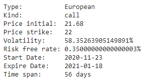
option_det = Option(european=True,
kind='call',
#change to put for put options
s0=21.68,
k=22,
t=56,
sigma=implied_volatility,
r=0.0035,
dv=0)
option_detAs can be seen we are looking at call options of Air Canada, with a strike price of $22, when the shares were trading at $21.68, with 56 days to maturity. The risk free rate used here is .35% with a dividend yield of 0%.
The code should spew out the following results –
We now move on to find out the price of the contract for which the code is as follows –
#Black Scholes Model (More Iterations = More accuracy), others are monte carlo and binomial tree
price0 = option_det.getPrice(method='BSM',iteration=5000)
mcprice = option_det.getPrice(method='MC',iteration=5000)
btprice = option_det.getPrice(method='BT',iteration=5000)
avg = statistics.mean([btprice,price0,mcprice])
print('BSM Price is '+str(price0), ', MC Price is ' +str(avg), ', BT Price is ' +str(btprice))
print('Average Price is ' +str(avg))
As we can see, I have used three different models and also printed the average pricing of the three in addition to the individual prices. Do note that there are likely to be minor pricing variations depending on the number of iterations run. This process is also resource heavy, especially with a high number of iterations.

Checking Profit & Loss
Now that we have the prices and are willing to purchase the contracts, we calculate the stock prices at which we are likely to break even, be in the red or make a profit. The gist of the code is that I have calculated the underlying contract premiums for a range of underlying prices, and then extrapolated the pricing difference between these prices to calculate the profit and loss. For this article, I have considered one contracts to include 100 shares with commission fees of $10 per trade + 1$ per contract.
from optionprice import Option
ploss = {'Equity Market Price': [smp-3,smp-2,smp-1,smp,smp+1,smp+2,smp+3]}
noc = 2 #number of contracts bought/sold
sperc = 100*noc #100 shares per contract
df = pd.DataFrame(ploss, columns = ['Equity Market Price','Profit/Loss'])
cpt = 10 + noc #commissions per trade, here assumed $10 flat + 1$ per contract
pnl=[]
for i in df['Equity Market Price']:
  option_det = Option(european=True,
                    kind='call',
                    s0=i,
                    k=22,
                    t=56,
                    sigma=implied_volatility,
                    r=0.0035,
                    dv=0)
  price = option_det.getPrice(method='BSM',iteration=5000)
  pnl.append(((price-price0)*(sperc))-(cpt*2))

ploss['Profit/Loss']=pnl
final=pd.DataFrame(ploss,columns=['Equity Market Price','Profit/Loss'])
#Note that calculations may not show zero value for options at purchase price view iterations differences
print(final) 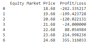
Plotting a graph, we get –
import matplotlib.pyplot as plt
plt.axhline(0, color='black', linestyle='solid', linewidth=1)
plt.plot(final['Equity Market Price'],final['Profit/Loss'])
plt.title('Option Profit and Loss Graph')
plt.xlabel('$Equity Price')
plt.ylabel('$Profit / Loss')
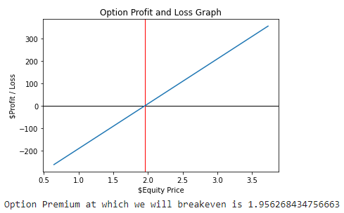
plt.show()beven = (price0*sperc+(cpt*2))/sperc
plt.axhline(0, color='black', linestyle='solid', linewidth=1)
plt.axvline(beven, color='red', linestyle='solid', linewidth=1)
plt.plot(final['Option Premium'],final['Profit/Loss'])
plt.title('Option Profit and Loss Graph')
plt.xlabel('$Equity Price')
plt.ylabel('$Profit / Loss')
plt.show()
print('Option Premium at which we will breakeven is ' +str(beven))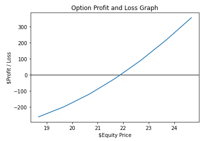
Conclusion
Hope this exercise has been helpful, and that this has stoked some of your curiosity in this space. Feel free to explore this model in tandem with optimizing your portfolio and thereafter calculating its VaR!
Please do not treat this article as investment or expert advise. All views expressed as personal. Feel free to reach out to me on LinkedIn or Twitter and comment on my articles!