Compute optimized asset weights and allocation for your portfolio using the modern portfolio theory in Python

Modern Portfolio Theory — (MPT)
Modern Portfolio Theory (MPT) or mean-variance analysis is a mathematical model/study for developing and creating a portfolio which aims to maximize the return for a given amount of risk. The math is largely based on the assumption and experience that an average human prefers a less risky portfolio. The risk mitigation can be done by either investing in traditional safe havens or by diversification — a cause championed by the MPT.
The theory was introduced by Henry Markowitz in the 1950s, for which he was awarded the Nobel prize. While the MPT has had its fair share of criticisms, partly due to its backward looking tendencies and inabilities to factor in force majeures/trends in business and economy, I find the tool valuable to gauge the risk of one’s portfolio holdings by measuring the volatility as a proxy.
Basics of the Model
I will be using Python to automate the optimization of the portfolio. The concepts of the theory are mentioned below in brief:-
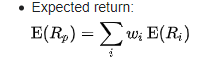
- Portfolio Expected Return –
The expected return of a portfolio is calculated by multiplying the weight of the asset by its return and summing the values of all the assets together. To introduce a forward looking estimate, probability may be introduced to generate and incorporate features in business and economy.
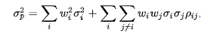
2. Portfolio Variance –
Portfolio variance is used as the measure of risk in this model. A higher variance will indicate a higher risk for the asset class and the portfolio. The formula is expressed as
3. Sharpe Ratio
The Sharpe ratio measures the return of an investment in relation to the risk-free rate (Treasury rate) and its risk profile. In general, a higher value for the Sharpe ratio indicates a better and more lucrative investment. Thus if comparing two portfolio’s with similar risk profiles, given all else equal it would be better to invest in the portfolio with a higher Sharpe Ratio.

4. The Efficient Frontier –
This plot measure risk vs returns and is used to select the most optimum portfolio to invest into after considering the risk profile and the characteristics of the investor. The efficient frontier is essential the part of the curve in the first and second quadrants depending on the objective and investor ability/characteristics.
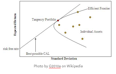
The Capital Allocation Line (CAL) is essentially a tangent to the efficient frontier. The point of intersection between the tangent and the frontier is considered to be the optimal investment which has maximum returns for a given risk profile, under normal conditions
Automating Portfolio Optimization in Python
- Importing Libraries
We will first import all the relevant libraries to help make our life easier as we progress.
#Importing all required libraries
#Created by Sanket Karve
import matplotlib.pyplot as plt
import numpy as np
import pandas as pd
import pandas_datareader as web
from matplotlib.ticker import FuncFormatter
Additionally, a critical library is the PyPortfolioOpt which contains functions to help us with the optimization of the portfolio. We will install the library with the following commands
!pip install PyPortfolioOpt
#Installing the Portfolio Optimzation Library
Import the functions which will be required further on –
from pypfopt.efficient_frontier import EfficientFrontier
from pypfopt import risk_models
from pypfopt import expected_returns
from pypfopt.cla import CLA
from pypfopt.plotting import Plotting
from matplotlib.ticker import FuncFormatter
2. Scrapping Stock and Financial Data from the Web
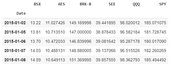
We will pull data from Yahoo! Finance for various stock tickers. The tickers I have used are Boston Scientific, Berkshire Hathway, Invesco Trust, S&P Index Fund, AES Corp., and Sealed Air Corp. The tickers have been chosen to spread the investment across various industries.
After inputting the tickers, we need to create a blank dataframe which will be used to capture all the prices of the stocks via a loop. For the purpose of this exercise, I have filtered down to capture the Adjusted Close value of the stocks that we are studying.
tickers = ['BSX','AES','BRK-B','SEE','QQQ','SPY']
thelen = len(tickers)
price_data = []
for ticker in range(thelen):
prices = web.DataReader(tickers[ticker], start='2015-01-01', end = '2020-06-06', data_source='yahoo')
price_data.append(prices.assign(ticker=ticker)[['Adj Close']])
df_stocks = pd.concat(price_data, axis=1)
df_stocks.columns=tickers
df_stocks.head()
Check if any values captured are ‘NaN’. Of less importance will be zero values. In case, there are NaN values — good practice will be to either consider a different time series or fill in the data with the average price of D-1, D+1. In case of a large void I would prefer not considering and deleting the time series data rather than inserting a zero value.
#Checking if any NaN values in the data
nullin_df = pd.DataFrame(df_stocks,columns=tickers)
print(nullin_df.isnull().sum())
3. Calculations
We will move ahead with the calculations for the optimization of the portfolio. Start with capturing the expected return and the variance of the portfolio chosen.
#Annualized Return
mu = expected_returns.mean_historical_return(df_stocks)
#Sample Variance of Portfolio
Sigma = risk_models.sample_cov(df_stocks)
Proceed by computing and storing the values for a portfolio weight with maximum Sharpe ratio and minimum volatility respectively.
#Max Sharpe Ratio - Tangent to the EF
ef = EfficientFrontier(mu, Sigma, weight_bounds=(-1,1)) #weight bounds in negative allows shorting of stocks
sharpe_pfolio=ef.max_sharpe() #May use add objective to ensure minimum zero weighting to individual stocks
sharpe_pwt=ef.clean_weights()
print(sharpe_pwt)
This will provide you the weight of different holdings. In case you want to minimize ‘zero’ holding or weight feel free to use L2 regression. Additionally, the weight_bounds have been set from -1 to 1 for allowing computation of ‘shorting’ stocks. The same exercise will be undertaken for the minimum variance portfolio.

4. Plotting the Efficient Frontier and Optimizing Portfolio Allocation
The final step is the plot the efficient frontier for visual purposes, and calculate the asset allocation (i.e. no of shares to purchase or short) for a given dollar amount of a portfolio. For the purpose of this exercise, I have considered $10,000 — the default starting value on investopedia.

latest_prices = discrete_allocation.get_latest_prices(df_stocks)
# Allocate Portfolio Value in $ as required to show number of shares/stocks to buy, also bounds for shorting will affect allocation
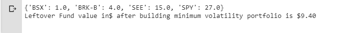
#Min Volatility Portfolio Allocation $10000
allocation_minv, rem_minv = discrete_allocation.DiscreteAllocation(minvol_pwt, latest_prices, total_portfolio_value=10000).lp_portfolio()
print(allocation_minv)
print("Leftover Fund value in$ after building minimum volatility portfolio is ${:.2f}".format(rem_minv))
This will provide you with the optimized portfolio as seen below
The same can be done for calculating the portfolio with the maximum Sharpe ratio.
Conclusion
Investing is said to be part art part science. Python and its libraries allow us to automate optimization and save valuable time in the process of doing so. However, it must be noted that these techniques in isolation are unlikely to be the best way to approach investing.
Moving ahead, I will post about how we can choose stocks to replicate an index fund via machine learning to build our portfolio and many other functions which Python can assist us with. Finally, I have also created a program to calculate potential losses or variations in share prices using monte carlo simulations. This tool may be used in tandem with this portfolio optimizer.
The information above is in no means expert investment advise or practices and is merely an effort by the me discuss how Python can be used to automate portfolio optimization via the Modern Portfolio Theory (MPT). For the complete source code or for any discussion, feel free to reach out
Pingback: Automating Option Pricing Calculations | Sanket Karve