Calculating Value at Risk (VaR) to manage financial risk of a portfolio using Monte Carlo Simulations in Python
VaR in Financial and Portfolio Risk Management?
VaR is an acronym of ‘Value at Risk’, and is a tool which is used by many firms and banks to establish the level of financial risk within its firm. The VaR is calculated for an investments of a company’s investments or perhaps for checking the riks levels of a portfolio managed by the wealth management branch of a bank or a boutique firm.
The calculation may be thought of as a statistical measure in isolation. It can also be simplified to the following example statement –
VaR is the minimum loss which will be incurred at a certain level of probability (confidence interval) OR the maximum loss which will be realized at a level of probability.
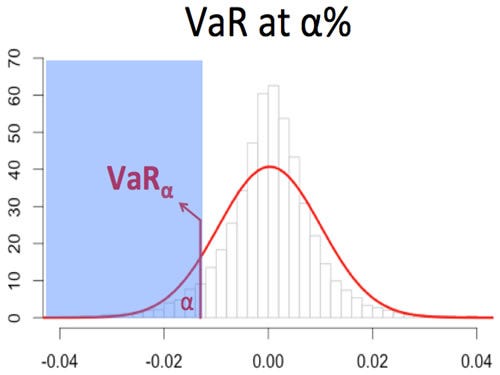
The above image shows the maximum loss which can be faced by a company at a α% confidence. On a personal level VaR can help you predict or analyse the maximum losses which your portfolio is likely to face — this is something which we will analyse soon.
Monte Carlo Simulations
The Monte Carlo model was the brainchild of Stanislaw Ulam and John Neumann, who developed the model after the second world war. The model is named after a gambling city in Monaco, due to the chance and random encounters faced in gambling.
The Monte Carlo simulation is a probability model which generates random variables used in tandem with economic factors (expected return, volatility — in the case of a portfolio of funds) to predict outcomes over a large spectrum. While not the most accurate, the model is often used to calculate the risk and uncertainty.
We will now use the Monte Carlo simulation to generate a set of predicted returns for our portfolio of assets which will help us to find out the VaR of our investments.
Calculating VaR in Python
We will first set up the notebook by importing the required libraries and functions
#Importing all required libraries
#Created by Sanket Karve
import matplotlib.pyplot as plt
import numpy as np
import pandas as pd
import pandas_datareader as web
from matplotlib.ticker import FuncFormatter
!pip install PyPortfolioOpt
#Installing the Portfolio Optimzation Library
from pypfopt.efficient_frontier import EfficientFrontier
from pypfopt import risk_models
from pypfopt import expected_returns
from matplotlib.ticker import FuncFormatter
For the purposes of our project, I have considered the ‘FAANG’ stocks for the last two years.
tickers = ['GOOGL','FB','AAPL','NFLX','AMZN']
thelen = len(tickers)
price_data = []
for ticker in range(thelen):
prices = web.DataReader(tickers[ticker], start='2018-06-20', end = '2020-06-20', data_source='yahoo')
price_data.append(prices[['Adj Close']])
df_stocks = pd.concat(price_data, axis=1)
df_stocks.columns=tickers
df_stocks.tail()
For the next step, we will calculated the portfolio weights of each asset. I have done this by using the asset weights calculated for achieving the maximum Sharpe Ratio. I have posted the snippets of the code for the calculation below.
#Annualized Return
mu = expected_returns.mean_historical_return(df_stocks)
#Sample Variance of Portfolio
Sigma = risk_models.sample_cov(df_stocks)
#Max Sharpe Ratio - Tangent to the EF
from pypfopt import objective_functions, base_optimizer
ef = EfficientFrontier(mu, Sigma, weight_bounds=(0,1)) #weight bounds in negative allows shorting of stocks
sharpe_pfolio=ef.max_sharpe()
#May use add objective to ensure minimum zero weighting to individual stocks
sharpe_pwt=ef.clean_weights()
print(sharpe_pwt)

The asset weights will be used to calculate the expected portfolio return.
#VaR Calculation
ticker_rx2 = []
#Convert Dictionary to list of asset weights from Max Sharpe Ratio Portfolio
sh_wt = list(sharpe_pwt.values())
sh_wt=np.array(sh_wt)
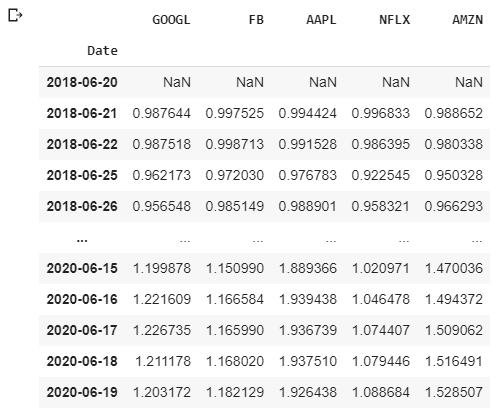
Now, we will convert the stock prices of the portfolio to a cumulative return, which may also be considered as the holding period returns (HPR)for this project.
for a in range(thelen):
  ticker_rx = df_stocks[[tickers[a]]].pct_change()
  ticker_rx = (ticker_rx+1).cumprod()
  ticker_rx2.append(ticker_rx[[tickers[a]]])
ticker_final = pd.concat(ticker_rx2,axis=1)
ticker_final
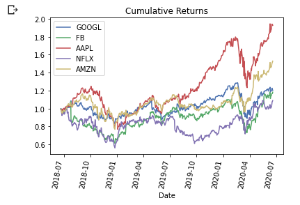
#Plot graph of Cumulative/HPR of all stocks
for i, col in enumerate(ticker_final.columns):
  ticker_final[col].plot()
plt.title('Cumulative Returns')
plt.xticks(rotation=80)
plt.legend(ticker_final.columns)
#Saving the graph into a JPG file
plt.savefig('CR.png', bbox_inches='tight')
Now, we will pick out the latest HPR of each asset and multiply the returns with the calculated asset weights using the .dot() function.
#Taking Latest Values of Return
pret = []
pre1 = []
price =[]
for x in range(thelen):
  pret.append(ticker_final.iloc[[-1],[x]])
  price.append((df_stocks.iloc[[-1],[x]]))
pre1 = pd.concat(pret,axis=1)
pre1 = np.array(pre1)
price = pd.concat(price,axis=1)
varsigma = pre1.std()
ex_rtn=pre1.dot(sh_wt)
print('The weighted expected portfolio return for selected time period is'+ str(ex_rtn))
#ex_rtn = (ex_rtn)**0.5-(1) #Annualizing the cumulative return (will not affect outcome)
price=price.dot(sh_wt) #Calculating weighted value
print(ex_rtn, varsigma,price)
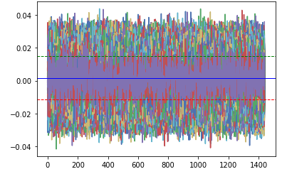
Having calculated the expected portfolio return and the volatility (standard deviation of the expected returns), we will set up and run the Monte Carlo simulation. I have used a time of 1440 (no of minutes in a day) with 10,000 simulation runs. The time-steps may be changed per requirement. I have used a 95% confidence interval.
from scipy.stats import norm
import math
Time=1440 #No of days(steps or trading days in this case)
lt_price=[]
final_res=[]
for i in range(10000): #10000 runs of simulation
  daily_return=                     (np.random.normal(ex_rtn/Time,varsigma/math.sqrt(Time),Time))
  plt.plot(daily_returns)
plt.axhline(np.percentile(daily_returns,5), color='r', linestyle='dashed', linewidth=1)
plt.axhline(np.percentile(daily_returns,95), color='g', linestyle='dashed', linewidth=1)
plt.axhline(np.mean(daily_returns), color='b', linestyle='solid', linewidth=1)
plt.show()
Visualizing the distribution plot of the returns presents us with the following chart
plt.hist(daily_returns,bins=15)
plt.axvline(np.percentile(daily_returns,5), color='r', linestyle='dashed', linewidth=2)
plt.axvline(np.percentile(daily_returns,95), color='r', linestyle='dashed', linewidth=2)
plt.show()
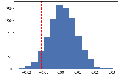
Printing the exact values at both the upper limit and lower limit and assuming our portfolio value to be $1000, we will calculated an estimate of the amount of funds which should be kept to cover for our minimum losses.
print(np.percentile(daily_returns,5),np.percentile(daily_returns,95)) #VaR - Minimum loss of 5.7% at a 5% probability, also a gain can be higher than 15% with a 5 % probability
pvalue = 1000 #portfolio value
print('$Amount required to cover minimum losses for one day is ' + str(pvalue* - np.percentile(daily_returns,5)))

The resulting amount will signify the dollar amount required to cover your losses per day. The result can also be interpreted as the minimum losses that your portfolio will face with a 5% probability.
Conclusion
The method above has shown how we can calculate the Value at Risk (VaR) for our portfolio. For a refresher on calculating a portfolio for a certain amount of investment using the Modern Portfolio Thoery (MPT), will help to consolidate your understanding of portfolio analysis and optimization. Finally, the VaR, in tandem with Monte Carlo simulation model, may also be used to predict losses and gains via share prices. This can be done by multiplying the daily return values generated with the final price of the respective ticker.
All views expressed are my own. This article is not to be treated as expert investment advise.
Feel free to reach out to me on LinkedIn and drop me a message
Pingback: Automating Option Pricing Calculations | Sanket Karve